How the Kalman Filter Powers Modern Quantitative Finance
When you hear “Kalman filter,” your mind might wander to spacecraft navigation or signal processing. Yet the same recursive algorithm is quietly reshaping trading floors, risk desks, and algorithmic research labs. Its charm lies in a simple promise: blend noisy observations with a model of how the world moves, and you get a clearer estimate of the hidden state. In finance, that hidden state is often the true price, volatility, or even the drift of an asset hidden beneath market chatter.
Why the Kalman filter fits finance so well
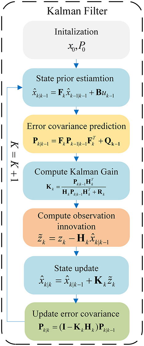
Markets are messy. Prices bounce, spreads widen, and data streams arrive at irregular intervals. Classical statistical tools—like moving averages—smooth but ignore the underlying dynamics. The Kalman filter, by contrast, assumes a state‑space model:
- State equation: how the hidden variable (say, the true asset value) evolves over time.
- Observation equation: how the market price you see relates to that hidden value, plus measurement noise.
This separation lets you treat market micro‑noise as just another source of error, rather than something to be filtered out manually. The result is a real‑time estimate that adapts as new quotes arrive, without the lag of a simple moving average.
Building a basic finance model with the filter
Consider a single‑asset price process. A common choice is the discrete‑time random walk:
xₜ₊₁ = xₜ + wₜ, where xₜ is the hidden true log‑price and wₜ ~ N(0,Q) captures the asset’s intrinsic volatility.
The observable price yₜ is then:
yₜ = xₜ + vₜ, with vₜ ~ N(0,R) representing market microstructure noise (bid‑ask bounce, latency, etc.).
Feed these equations into the filter and you obtain an optimal linear estimator for xₜ. In practice, you calibrate Q and R from historical variance and observed tick‑level noise, then let the recursion handle everything else.
Extensions that matter to quants
Time‑varying volatility
The vanilla filter assumes constant Q and R, but real markets roar and lull. A popular tweak is the “switching Kalman filter,” where you let Q change depending on a volatility regime indicator (e.g., high‑vol vs. low‑vol states). The filter then automatically picks the appropriate level of smoothing.
Non‑linear dynamics
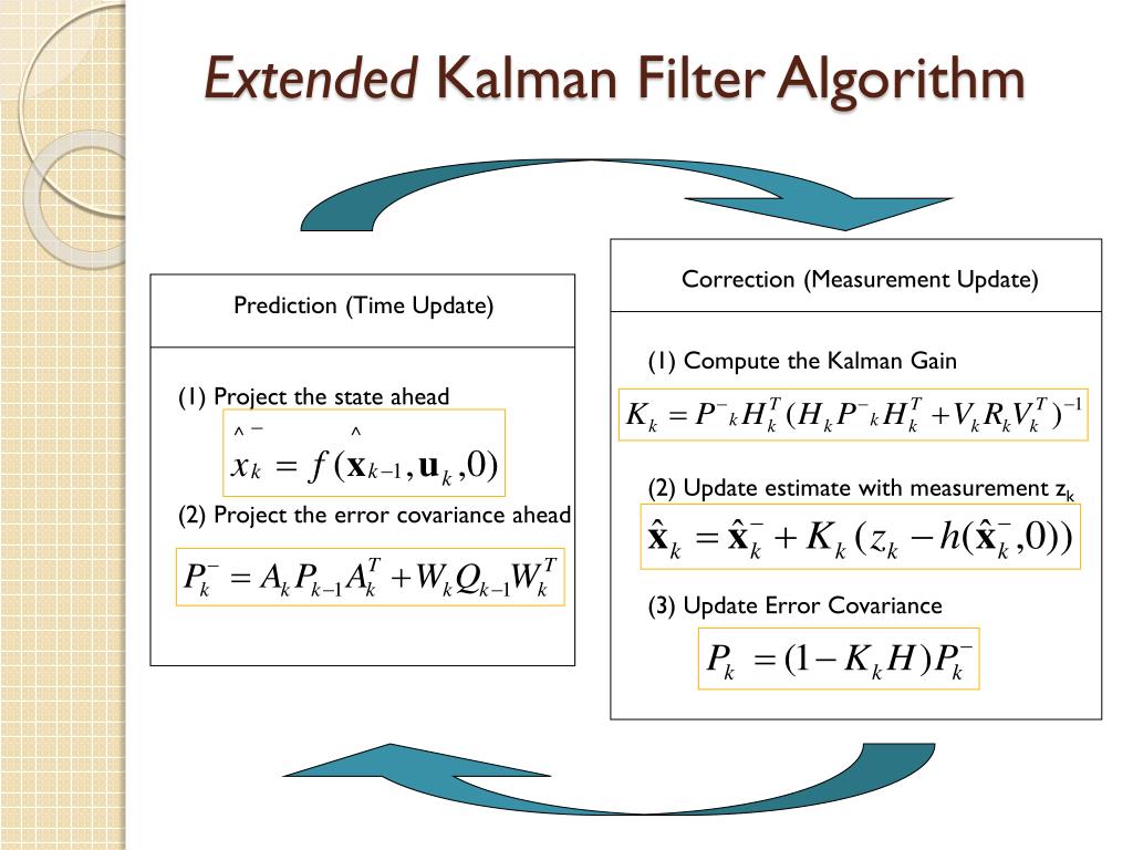
Assets sometimes follow drift‑diffusion models that aren’t linear. The extended Kalman filter (EKF) linearizes around the current estimate, while the unscented Kalman filter (UKF) uses a deterministic sampling scheme to capture non‑linearity more faithfully. Both have found niche use in options pricing where the underlying follows stochastic volatility dynamics.
Multivariate assets
Portfolio managers love to track correlated securities. By stacking each asset’s state into a single vector, the filter can jointly estimate a covariance matrix that evolves over time. This yields a dynamic risk model that reacts instantly to a shock in one market, adjusting exposures across the board.
Real‑world applications on the trading floor
High‑frequency signal extraction: Market makers feed raw tick data into a Kalman filter to separate the “true” mid‑price from transient noise, allowing them to post tighter quotes without getting whipsawed.
Statistical arbitrage: Pairs‑trading strategies often model the spread between two stocks as a mean‑reverting process. The Kalman filter continuously estimates the spread’s equilibrium level, flagging deviations that could be exploited.
Dynamic hedging: For options desks, the Greeks (Delta, Gamma) shift as volatility morphs. A Kalman filter applied to implied volatility surfaces delivers smoother, lag‑free updates, making delta‑hedging more precise.
Pitfalls and practical tips
Even a powerful tool can misbehave if you ignore its assumptions. First, the filter is optimal only under Gaussian noise. Heavy‑tailed jumps—think flash crashes—can throw the estimator off. Remedies include robust variants that downweight outliers or simply resetting the filter after a detected shock.
Second, the choice of initial conditions matters. A wildly inaccurate initial state variance can cause the filter to over‑react or stay stuck. A common practice is to run a short “burn‑in” period using a simpler estimator, then hand the calibrated state to the Kalman recursion.
Finally, computational speed is rarely a deal‑breaker for a single asset, but multivariate models can balloon in dimension. Sparse matrix techniques and parallel processing keep the filter usable for portfolios of hundreds of securities.
Getting started yourself
If you’re curious to experiment, most quantitative libraries already ship a Kalman implementation. In Python, filterpy or statsmodels provide ready‑made classes—just plug in your state and observation matrices. In R, the dlm package does the same. Begin with a simple random‑walk model, calibrate Q and R from a calm period, then watch how the estimate behaves during a volatile day.
As you grow comfortable, layer in regime‑switching or extend to a multivariate framework. The learning curve is gentle, but the payoff can be substantial: cleaner signals, faster reaction times, and a mathematically grounded way to navigate noisy markets.
In short, the Kalman filter isn’t a silver bullet, but it is a remarkably adaptable microscope for peering through market noise. Whether you’re a quant building a high‑frequency strategy or a risk manager seeking a real‑time volatility gauge, the filter offers a principled, data‑driven path to better decisions.