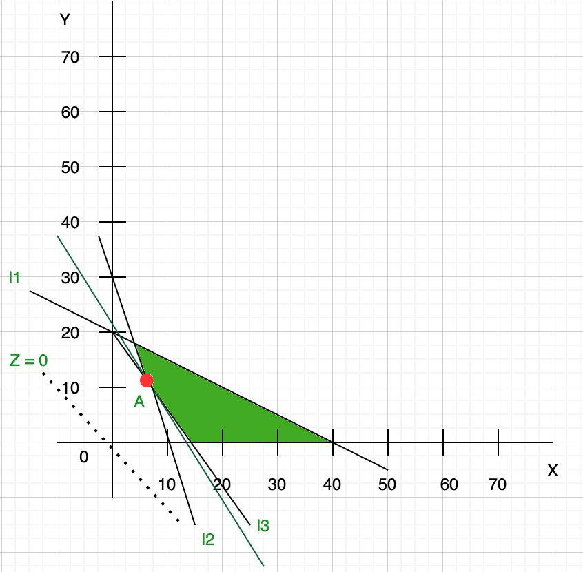
How to Solve Linear Programming Using the Graphical Method

Understanding the Basics

Linear programming (LP) is all about finding the best outcome—maximum profit or minimum cost—subject to a set of linear constraints. When the problem involves only two decision variables, the graphical method becomes a surprisingly visual and intuitive tool. Instead of diving straight into matrices and simplex tables, you literally draw the solution space on a piece of graph paper (or a digital plot) and let the geometry do the heavy lifting.

Formulating the Objective and Constraints

The first step is to translate the real‑world scenario into a mathematical model. You’ll end up with:

• An objective function—for example, maximize Z = 3x + 5y or minimize C = 2x + 4y.
• Several linear constraints—inequalities that bound the feasible region, such as 2x + y ≤ 20, x ≥ 0, and y ≥ 0.

Notice the non‑negativity restrictions; they keep the problem in the first quadrant, which is where the graphical method shines.

Converting Inequalities to Equalities

To draw each constraint, treat the inequality as an equation first. For 2x + y ≤ 20, rewrite it as 2x + y = 20. Plot the line by finding two convenient points—say, set x = 0 to get y = 20, then set y = 0 to get x = 10. Connect the dots, and you have the boundary line.

After all lines are on the graph, decide which side of each line satisfies the original inequality. A quick test point like (0,0) works for most cases; if it makes the inequality true, shade that side.

Drawing the Feasible Region

The feasible region is the intersection of all shaded halves. It’s typically a convex polygon—sometimes a triangle, rectangle, or irregular shape with up to six sides. Remember:

• If any constraint is a “≥” inequality, you’ll shade opposite the test point.
• When constraints are parallel, you might end up with no feasible region at all—an indicator that the model needs revisiting.

Once the region is clear, the optimal solution will sit at one of its corner (vertex) points. This is a direct consequence of the linear nature of the objective function.

Locating the Corner Points

Corner points arise where two constraint lines intersect. Solve each pair of equations simultaneously:

• For 2x + y = 20 and x + 3y = 15, subtract or substitute to find (x, y).
• Don’t forget the axes intersections—points where a constraint meets x = 0 or y = 0.

It’s easy to miss a vertex, especially when constraints overlap. Double‑check by plugging the coordinates back into all original inequalities.

Evaluating the Objective Function

Now the fun part: calculate the objective value at each vertex. Using the earlier example, if one corner is (5,10), compute Z = 3(5) + 5(10) = 65. Do this for every feasible corner, then compare:

• The highest Z (for a maximization problem) gives the optimal solution.
• The lowest Z (for a minimization problem) does the same.

Because the feasible region is convex, you’ll never find a better solution inside the region—only at the edges.

Interpreting the Result

Suppose the best corner is (4,6) with Z = 42. That tells you to produce 4 units of product A and 6 units of product B to achieve the maximum profit of 42 (in whatever monetary units you’re using). Also, note the “shadow price” concept: the slope of the objective line at that point hints at how sensitive the optimum is to changes in coefficients.

Common Pitfalls and How to Avoid Them

Missing a Constraint – Forgetting to plot a boundary line can make the feasible region appear larger, leading to an unrealistic optimum.

Wrong Shading Direction – Always test a point not on the line; the origin works unless the constraint itself passes through it.

Parallel Constraints – If two constraints are parallel and the feasible region collapses into a line, the optimum may lie anywhere along that line. In such cases, you’ll need additional criteria or a different method.

Numerical Errors – When solving for intersections, small arithmetic slips can shift a vertex outside the feasible region. Double‑check arithmetic or use a calculator.

When to Move Beyond the Graphical Method

The graphical technique shines for quick, two‑variable problems—think introductory economics or simple production planning. As soon as you add a third decision variable, you’re forced into three‑dimensional visualizations that quickly become unwieldy. At that point, the simplex algorithm or modern solver software takes over. Still, mastering the graph helps you develop intuition about feasibility, binding constraints, and the geometry behind LP.

Quick Reference Checklist

• Write the objective function and constraints clearly.
• Convert each inequality to an equality for plotting.
• Plot lines, test points, and shade correctly.
• Identify all feasible vertices by solving line intersections.
• Calculate the objective at each vertex.
• Select the maximum (or minimum) value.
• Validate the solution against all original constraints.