How to Use Currency Functions in Google Sheets: A Complete Guide

Ever stared at a spreadsheet full of numbers and wondered how to turn raw figures into neatly formatted currency? Google Sheets has a handful of tools that make this surprisingly painless. In this walk‑through we’ll explore the built‑in functions, formatting tricks, and a few quick formulas that let you handle dollars, euros, yen—or any symbol you need—without breaking a sweat.

Why Currency Formatting Matters

Beyond the visual polish, proper currency formatting helps prevent costly mistakes. A column of plain numbers can be misread, especially when dealing with large datasets or international partners. By attaching the right symbol and decimal precision, you instantly signal the value’s meaning and improve the sheet’s credibility.

Getting Started: Basic Number Formatting

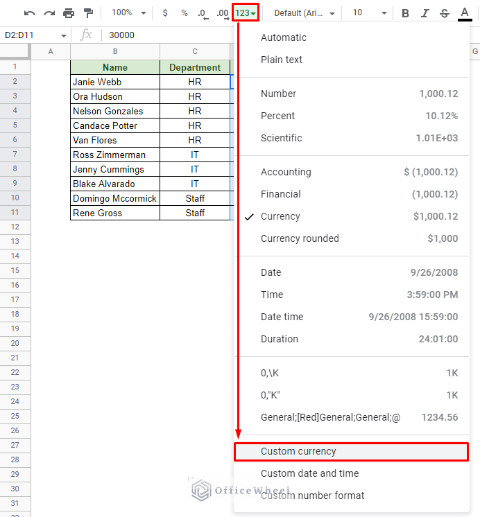
Google Sheets’ Format → Number → Currency menu does the heavy lifting for most cases. Here’s what happens when you apply it:

• The chosen currency symbol appears before the number.
• Two decimal places are added automatically.
• Negative values turn red (or whatever your theme dictates).

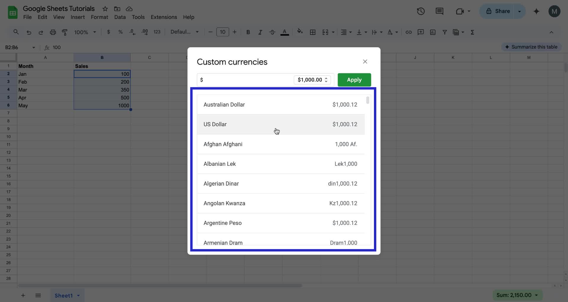
If you need a different currency, click More formats → Custom number format and type something like [$€-2]#,##0.00. The code tells Sheets to use the euro sign and keep the usual thousands separator.

Dynamic Currency Symbols with the TEXT Function

Static formatting works great for a single currency, but what if your sheet tracks sales across several markets? The TEXT function lets you build a string that includes a variable symbol:

=TEXT(A2,"$#,##0.00")   // Dollar format
=TEXT(A2,"€#,##0.00")   // Euro format

To make it truly dynamic, combine it with a lookup table:

=TEXT(A2, VLOOKUP(B2, CurrencyMap!A:B, 2, FALSE))

Here B2 holds the currency code (e.g., “USD” or “JPY”), and CurrencyMap contains the appropriate formatting strings.

Converting Between Currencies

Google Sheets can pull live exchange rates using the GOOGLEFINANCE function. Though not a full‑blown financial platform, it’s handy for quick conversions.

=A2 * GOOGLEFINANCE("CURRENCY:USDEUR")   // Convert USD to EUR

Remember, the data refreshes every two minutes, so it’s good enough for budgeting but not for high‑frequency trading. If you need more accuracy, consider a dedicated API and the IMPORTJSON script.

Tips for Stable Conversions

• Lock the rate cell with an absolute reference ($B$1) if you plan to copy the formula across rows.
• Round the result to two decimals with ROUND(...,2) to avoid long float tails.
• Store the fetched rate in a separate “settings” sheet to keep the main data clean.

Handling Complex Scenarios

Some businesses need to display both the original amount and the converted value side by side. A simple concatenation does the trick:

=TEXT(A2,"$#,##0.00") & " (" & TEXT(A2 * $B$1, "€#,##0.00") & ")"

This yields something like $1,200.00 (€1,020.00), instantly showing the dual perspective without extra columns.

Common Pitfalls and How to Avoid Them

• Mixed Data Types: If a column mixes text and numbers, formatting will skip the text entries, leaving them blank. Clean the data first.
• Locale Settings: A sheet set to a European locale will use commas as decimal separators. Override this with a custom format if you need the US style.
• Hidden Characters: Copy‑pasting from PDFs can introduce non‑breaking spaces. Use TRIM and SUBSTITUTE to strip them out.

Quick Reference: Useful Formulas at a Glance

• Simple Currency Format: =TEXT(A2,"$#,##0.00")
• Dynamic Symbol Lookup: =TEXT(A2, VLOOKUP(B2, Map!A:B, 2, FALSE))
• Live Conversion Rate: =GOOGLEFINANCE("CURRENCY:USDEUR")
• Rounded Conversion: =ROUND(A2*$B$1,2)
• Dual Display: =TEXT(A2,"$#,##0.00") & " (" & TEXT(A2*$B$1,"€#,##0.00") & ")"

With these tools in your spreadsheet arsenal, you can turn any jumble of numbers into clear, professional‑looking financial data. Whether you’re tracking a global startup’s revenue or just budgeting a family vacation, Google Sheets’ currency features keep things tidy and trustworthy.