Why the ‘c’ Matters: Decoding the Y‑Intercept in y = mx + c

When you first meet the equation y = mx + c, the “c” might seem like just another letter tacked onto a line‑drawing formula. In reality, it’s the anchor that tells you where the line meets the vertical axis, and understanding it opens the door to a surprisingly rich set of geometric and practical insights.

What the Y‑Intercept Actually Is

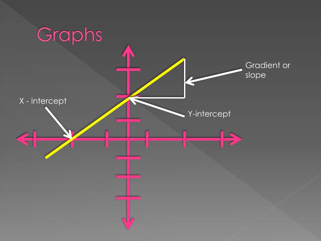
Think of a graph as a city map. The x‑axis runs east‑west, the y‑axis runs north‑south. The point where a road (your line) crosses the y‑axis is the “y‑intercept.” In algebraic terms, it’s the value of y when x = 0. That number is what we label “c.”

• c = 0 – the line shoots straight through the origin.
• c > 0 – the line starts above the origin on the y‑axis.
• c < 0 – the line starts below the origin.

This simple piece of information tells you instantly where the line begins, even before you know how steep it climbs.

Why “c” Isn’t Just a Constant

If you treat c as a fixed, unchanging number, you miss the way it reshapes a line without altering its slope. Imagine you’re sliding a ruler up and down a wall: the angle stays the same, but the point where the ruler touches the floor changes. In the equation, that shift is captured by c.

That distinction becomes crucial in real‑world modelling. Suppose you’re tracking a car’s mileage over time. The slope m represents average miles per month; c tells you the starting mileage when you first logged the data. Change the starting point—perhaps you bought a new car—and c adjusts, while m remains the same if your driving habits don’t change.

Finding c From Data

Often you have a set of (x, y) points and need to uncover the underlying line. The traditional “two‑point form” works like this:

1. Pick any two points, (x₁, y₁) and (x₂, y₂).

2. Compute the slope: m = (y₂ − y₁)/(x₂ − x₁).

3. Substitute one point into y = mx + c and solve for c.

Because c is the y‑value when x = 0, you can also extrapolate directly: draw the line, follow it back to the y‑axis, and read off the intercept. In spreadsheet software, the “INTERCEPT” function does the heavy lifting, but the geometry remains the same.

c in Different Contexts

While algebra textbooks present c as a tidy constant, many fields give it a more descriptive name.

• Physics: In kinematics, y = vt + s₀, where s₀ (the initial position) plays the role of c.
• Economics: In cost analysis, total cost = variable cost × quantity + fixed cost. The fixed cost is the y‑intercept.
• Biology: Growth curves often start at a baseline population size—again, the y‑intercept.

Seeing c as “initial value,” “baseline,” or “fixed component” helps translate the math into everyday language.

When c Vanishes

A line that passes through the origin (c = 0) has a special symmetry: the graph is a straight line that scales directly with x. In proportional relationships—like speed = distance ÷ time—there’s no “starting offset.” If you encounter a dataset that looks almost proportional but not quite, a small non‑zero c may be the clue you need.

Graphical Tricks to Spot c Quickly

Sometimes you only have a rough sketch. Here are two quick visual cues:

• Horizontal shift test: Slide the line vertically until it hits the y‑axis; the distance moved equals c.
• Intercept comparison: If you have two lines with the same slope, the one higher on the y‑axis has a larger c.

These shortcuts save time when you’re troubleshooting a model or checking a colleague’s work.

Common Misconceptions

People often assume that c must be positive because it’s “above” the x‑axis. On the contrary, a negative c simply means the line begins below the origin—nothing mathematically illegal about that. Another myth is that c determines the line’s steepness; that’s the job of m. Change c, keep m, and the line slides up or down without tilting.

Using c to Translate Between Forms

Besides the slope‑intercept form, you might see the point‑slope version: y − y₁ = m(x − x₁). Convert it back by expanding and gathering terms; the constant term that surfaces is c. This back‑and‑forth helps when you’re given a point and a slope but need the full equation for a graphing calculator.

Real‑World Example: Budget Planning

Imagine a small business projects monthly revenue as R = 200 × m + c, where m is the number of marketing campaigns run per month. If historic data shows that running five campaigns yields $12,000, and ten campaigns brings in $22,000, you can solve:

m₁ = 5, R₁ = 12,000;

m₂ = 10, R₂ = 22,000.

The slope m = (22,000 − 12,000)/(10 − 5) = 2,000. Plugging back, 12,000 = 2,000·5 + c gives c = 2,000. That $2,000 represents baseline revenue without any marketing—perhaps recurring subscriptions or existing customers. Adjusting c (through price changes, for instance) directly lifts the whole revenue line without affecting how each campaign contributes.

Wrapping Up the Role of “c”

The humble “c” does more than sit at the end of an equation. It tells you where a line starts, anchors real‑world models, and offers a quick visual shortcut on a graph. Whether you’re a student sketching a line on notebook paper or a analyst forecasting sales, paying attention to the y‑intercept can save time, reveal hidden assumptions, and make your mathematical story clearer.